
The context for Power Pivot… If you are a frequent Excel user, then you are probably familiar with pivot tables. Pivot tables are used for figuring out quick insights from small amounts of data and can also be turned into easy to understand graphs.
But even Excel has its limitations.
When combining tables, manipulating large datasets over one million rows, or selecting data from multiple sources, Excel will struggle. It can be frustrating to have Excel quit unexpectedly or run extremely slowly or time out and need a forced shutdown!
So, what happens if you have over one million rows (1,048,576 to be exact) of data? You use Power Pivots.
In 2010 Microsoft added Power Pivots to Excel to help with the analysis of large amounts of data. Power Pivot can handle hundreds of millions of rows of data, making it a better alternative to Microsoft Access, which before Excel was the only way to accomplish it. Think of Power Pivot as a way to use pivot tables on very large datasets.
It is also helpful when data is coming from multiple sources. With Power Pivot, you can import that data into just one workbook without needing multiple source sheets, which can get confusing and frustrating.
Power Pivot was built to import and analyze data from multiple sources. Anything, from Microsoft SQL, Oracle, or Access databases, to SharePoint list data and text documents, can be used as data sources in Power Pivot.
Accessing Power Pivot
Power Pivot is a free add-in tool within Excel and is a permanent built-in feature in Excel 2016 and 365. The first step in using power pivot is adding it to your Excel ribbon. In recent versions of Microsoft Excel (13’ – 17’) Power Pivot is built in, but you may need to activate it.
Enable Power Pivot by clicking File -> Options -> Add-ins -> Microsoft Power Pivot for Excel:

Now Power Pivot is enabled, but not quite ready to use. There is still one more step.

You will need to tell Power Pivot where to go to import data. To do this, click on the Power Pivot tab in the ribbon -> Manage data -> Get external data. There are a lot of options in the Data Source list. This example will use data from another Excel file, so choose Microsoft Excel option at the bottom of the list. For large amounts of data, the import will take some time.

When the import is done, you will see the data in the main Power Pivot window. There will be two windows will open at the same time – the regular Excel window and the Power Pivot window. You do not need to have data in the opened Excel page, though.
Creating a Basic Power Pivot Table
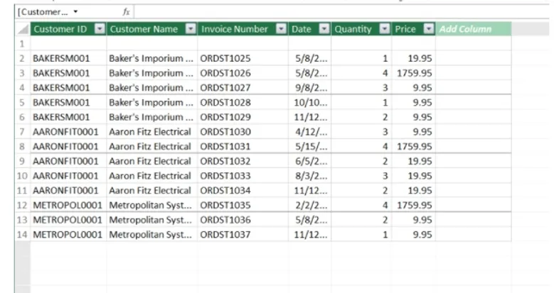
Let’s say you’ve got a spreadsheet that has a list of product sales. Each row is a Customer ID and the columns are Name, Invoice Number, Date, Quantity, and Price.

Because customers have more than one invoice but only one customer ID, customer information has to be repeated multiple times. This doesn’t seem like an issue when there are only a few invoices. But when the invoices start to add up to one million, it will be less efficient to use this format in basic Excel and more efficient to create a Power Pivot.
To do this, open a new Excel workbook. Choose Power Pivot from the ribbon, then click Manage -> From Other Sources and scroll down to Excel. On the screen, select the file using the Browse button.

Once the file is selected, click Next. It’s good to rename the “Friendly Name” header to a title that describes the data set. In this case, the title has been changed to “Invoices.” Click Finish.

Success! The list of invoices has been imported into a Power Pivot Table. From here, you can create Pivot Table charts just like you would with smaller data sets (explained in the next section). Again, the reason Power Pivot would be used here is if the data was in another format (SQL, Access, Oracle) or if there were over one million rows in an Excel file. Otherwise, using the basic Pivot Table function in Excel would work without error.

Creating a Pivot Chart from a Power Pivot Table
To create a chart from this Power Pivot, click the PivotTable icon in the Excel ribbon and choose Pivot Chart (choose PivotTable if you want to create a normal PivotTable in Excel first before creating a chart).

A new workbook will open. Use the fields toolbar on the right to select fields for the table. In this example, each company’s order is being compared month over month. So Customer Name, Date, and Quantity have been selected and included in the Pivot Chart.

Tip: Power Pivot Formulas
Power Pivot has a lot of nice features and perks. In addition to the normal Excel functions, it introduces over 75+ new formulas. Here are two good ones to know:
=COUNTROWS: Counts the number of rows in a data source. If you have multiple data sources that relate to each other by an ID, such as a product name, you can also count the number of rows in relation to those identifiers.
=SWITCH: Switch is incredibly useful for data that needs editing. For example, you might have rows with with a number indicating a certain month, instead of the month’s actual name – 1 for Jan, 2 for Feb, 3 for March, etc. Use =SWITCH to change (switch) all the numbers to the actual month.

Power Pivot automatically uses the =SUM calculation to summarize numeric data, which is a great feature. To change the type of calculation used, right click inside the pivot table and choose Value Field Settings -> Summarize Values by Tab. As you can see in the image, =COUNT, =AVERAGE, =MIN, =MAX and many others are options.

Tip: Power Pivot and SharePoint
Many organizations use Microsoft Sharepoint. Power Pivot dashboards, graphs, and pivot graphs can be published straight to Sharepoint for quick viewing by anyone in your organization. To use this, install the “Power Pivot for SharePoint” plug-in on your company Sharepoint site.
Power Pivots may seem like an advanced Excel function, but they are easy to use once you understand how to access the feature and import a data set. Once the data is in, you can run a PivotTable or Pivot Chart off the dataset like you would and normal table of data. Power Pivot is one of the quickest ways to provide you with easy insights into large amounts of data that might otherwise crash Excel or at a minimum drive you mad. So if you find yourself with millions of rows in a spreadsheet, find and use Power Pivot.
The Ideal match to Power Pivot
The best FP&A solution for Excel Users out there right now is DataRails. They collect, report, and analyze data with ease using the FP&A solution build for finance professionals. Without changing the way you work, you can build a unified database of all your numbers but automating the collection of data from each of your organizational systems and spreadsheets.
In conclusion, if you are a finance professional looking to make your life easier, you have to take a look at this platform.


