

Do you find yourself spending too much time formatting Excel sheets? Do you wish you could use your time better, but you’re not sure how? No worries! We have tips on how to format your Excel spreadsheets like a pro.
Whether you’re a beginner or an expert, these tips will enhance your data entry, make your reports look better, turn text into numbers, simplify complex formulas, and overall, make your data more organized and presentable.
How to Format Your Excel Spreadsheets?
In Excel, formatting means changing or organizing data in spreadsheets. You can modify how data looks and its type easily. After understanding the basics, you’ll now see how to do formatting as you work.
Excel formatting covers different needs like changing appearance, data type, and organization. To format data, go to the home tab in Excel.
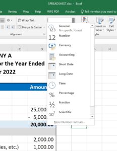
1. Number Formatting
Correct number formats are crucial as they ensure accurate reports. Let’s consider a practical example: imagine you’re tasked with identifying the customer who made the highest purchase in a month at an automotive store. The goal is to reward this customer with a discount on their next purchase.
Now, picture that all transactions are recorded in dollars except for one. Due to haste, you forgot to add the dollar format to the highest transaction of the month. This simple oversight can lead to complications.
To avoid such issues, it’s essential to understand number formatting in Excel and how to apply it correctly.
Follow these steps:
- Choose a cell, a range of cells, or an entire column where you want to apply number formats.
- Go to the Home button.
- In the Number Group, click the drop-down menu to access number formatting options.
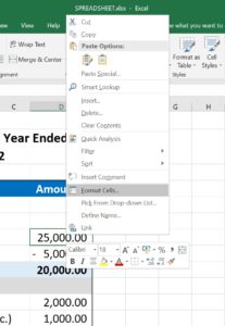
Here’s another method:
- Choose a cell, a group of cells, or a whole column.
- Right-click on the selected cell.
- A menu will appear.
- Open the Number Group and choose the drop-down for Number formatting.
Now that you’ve learned how to use Excel’s number formats, let’s explore the different formats you can use:
General
- The default format for any number input.
- No additional decimals or modifications.
Number
- Used exclusively for working with numbers.
- Adds decimal points for accuracy; customizable.
Currency
- Represents numbers as currency (e.g., dollars).
- Useful for financial data like annual investments.
Accounting
- Similar to currency; adds decimal places for accuracy.
Date
- Treats input as a calendar date instead of a regular number.
Time
- Converts default number format to time format.
Percentage
- Represents values as percentages (multiplied by 100).
- Displays decimal values in percentage format.
Fraction
- Displays numbers as fractions based on user choice.
Scientific
- Differs from other formats; includes exponential notation.
- Covers trigonometry, calculus, roots, etc.
Text
- Treats input as textual data; no decimals or symbols added.
Special
- Includes symbols alongside numbers, text, and scientific notations.
- Requires selecting the format for the special symbol.
Custom
- Excel allows users to customize existing formats or create new ones.
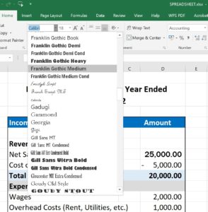
2. Cell Formatting
Formatting cells in Excel involves more than just changing numbers. It includes adjusting text alignment, color, font, cell background, and adding images.
To explore font options in Cell Formatting:
- Go to the Home tab.
- Find the Font group.
- Click the drop-down icon for a range of font choices.
Following the Font option, explore font color, bold, italic, and underline choices, as well as text alignment in the Home tab. On the right side in the alignment group, find text alignment, text wrapping, and text indentation options.
3. Text Color and Cell Color Formatting
The Text color feature lets users pick different colors for text in Excel, as seen below.
The Cell background color feature allows users to change the background color of cells in the spreadsheet, as shown below.

4. Cell Borders Formatting
The spreadsheet borders feature lets users easily add cell borders based on their needs.

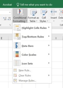
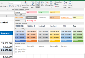
5. Conditional Formatting
Located to the right of the Number Format Group, you’ll find options for Conditional Formatting, Cell Formatting, and Table Formatting, as depicted below.
With Conditional Formatting, users can highlight or mark cells in Excel spreadsheets using logical functions and formulas, as demonstrated below.
6. Table Formatting
Excel’s Table Formatting enables you to change the layout of data in Excel using different options, as depicted in the image below.

7. Cell Formatting
The Cell Formatting feature lets users change the background color of specific cells according to their needs, as demonstrated below.
Handy Excel Formula for Basic Daily Transaction
In Excel, a formula is a way to do math on groups of cells. Formulas give you an answer, even if there’s an error. You can use formulas to add, subtract, multiply, and divide. You can also find averages, calculate percentages, work with dates and times, and more.
Excel has many formulas and functions for different tasks. We’ll explore basic ones for math, text, and common data operations. Using these formulas to format your Excel spreadsheet can be handy in everyday use.
Sum
The SUM() function adds up the values in a chosen range of cells, providing the total through addition.
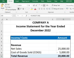
As shown earlier, to calculate the total sales for each unit, we just entered the formula “=SUM(D7:D8).” This formula adds up the numbers in cells D7 and D8, and the total is displayed in cell D9.
Average
The AVERAGE() function is used to find the average of a group of selected cells. For instance, if you want to find the average of total sales, just type: =AVERAGE(E5,E6,E7,E8,E9)
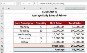
It will calculate the average for you, and you can save the result where you want.
Count
The COUNT() function tallies the cells within a range that has numerical values. It excludes empty cells and those with data in non-numeric formats.
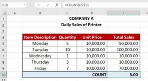
As shown earlier, we’re counting from E5 to E9, which has 5 cells. The COUNT function considers only cells with numbers, so the answer is 5, excluding the cell with “Total Sales.”
If you need to count all cells with any type of data (numbers, text, etc.), use the COUNTA() function. Note that COUNTA() doesn’t include blank cells.
To count blank cells in a range, you can use COUNTBLANK().
Subtotal
SUBTOTAL() provides the total value in a database, and you can choose from options like average, count, sum, min, max, and more, depending on your needs. Let’s examine two examples to understand better.
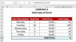
In the given example, we calculated the subtotal for cells C5 to C9. The function used is associated with “1” in the subtotal list, representing the average. Therefore, the function calculates the average of C5 to C9, resulting in an answer of 5, which is stored in cell E10.
Likewise, using =SUBTOTAL(4,E5:E9) picks the highest value from cells C5 to C9, which is 10. Including “4” in the function gives the maximum result.

Conclusion
Excel is recognized as a powerful spreadsheet tool specifically crafted for efficient data analysis and reporting. The provided examples of cell formatting and fundamental formulas will help you gain valuable insights into essential Excel formulas and functions, enabling you to perform tasks more efficiently and swiftly. Using tools, such as FP&A software, that are compatible with Excel will help you make even more efficient use of your Excel proficiency.


