
Say you have a table of data and you want Excel to look up a certain value and return a corresponding value in a different row. For that, you need a lookup function. Excel has a range of functions that you can use to achieve this including VLOOKUP() and HLOOKUP() and the more flexible, but slightly more complicated, combination of INDEX() and MATCH().
Although the Excel lookup functions can seem quite straightforward, it’s very easy to get the wrong answer if you don’t fully understand how they work. For those of you who aren’t already using Datarails to automate all of your finances, we wanted to show you how to do it manually.
Excel does have an additional lookup function: LOOKUP() but this is only included for compatibility with older spreadsheet applications, so we’ll concentrate on VLOOKUP() and HLOOKUP(). The V and H in the names of these two functions refer to Vertical and Horizontal respectively, so the good news is that once you’ve learnt how to use VLOOKUP(), HLOOKUP() should be easy, as it works in exactly the same way, but with data arranged in rows as opposed to columns.
VLOOKUP()
The VLOOKUP() function assumes that your data is arranged as a table with different elements of the information in different columns.
If we need to return multiple results from a table then the lookup functions are unlikely to work. You would either need to filter the table or use a PivotTable.
APPROXIMATE MATCH
Let’s now look at an even more important issue with the lookup functions. The use of the optional, fourth argument. Perhaps we don’t know about the fourth argument or we aren’t sure about the spelling of ‘Lotta’ so we think we’ll use an approximate match rather than an exact match:
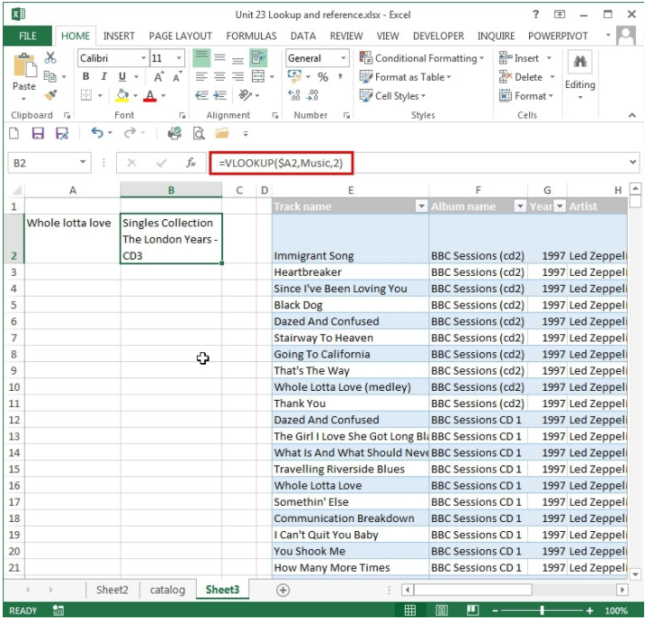
All we have changed in our formula is to omit the fourth argument. Although there are several exact matches for our value in our table, the function now returns a completely different album title. In fact, a Rolling Stones album that certainly doesn’t include Led Zeppelin’s ‘Whole Lotta Love’. If we changed our column index to 1, we would find that Excel had matched ‘Whole Lotta Love’ with ‘Honky Tonk Women’.
So something isn’t right…
The reason for this is that the approximate match doesn’t mean find the ‘closest’ value to our lookup value wherever it is in the table. It is actually a much more specific type of match than that:
it finds the largest value in our table that is smaller than, or equal to, our lookup value. In fact, it’s really even more specific than that. If there is no exact match, it will find the first item in our table larger than the lookup value and match with the cell immediately above.
For this reason, whenever you don’t specify an exact match by using FALSE as the fourth argument in VLOOKUP(), you must ensure that your table of data is sorted in ascending order, using the leftmost column.
Here, we have re-sorted our table and used two approximate matches, and two exact matches, all referring to columns 1 and 2. For two of our formulae, we have entered an inexact track name (‘Whole lot of love’). Where there is a match, we have positioned the VLOOKUP() statement next to the row it matches:

You can see that:
- Where there is no exact match, and exact is specified by entering FALSE as the fourth argument, the formula returns a #N/A error.
- Where there is no exact match and the fourth argument is omitted or TRUE is used, VLOOKUP() finds the first item ‘larger’ than our lookup value and uses the cell immediately above.
- Where there is an exact match and exact is specified, the first match from the top is found.
- Where there is an exact match and exact is not specified, the first match from the bottom is found.
- In case you were wondering why ‘Whole lotta love’ is ‘larger’ than ‘Whole lot of love’: they are the same up until the first t, then for the next character, the letter t has a higher value when sorting letters than a space.
To be honest, the majority of times you use a VLOOKUP, you will be looking for an exact match. So you would be forgiven for wondering what the point of an approximate match is. They can be very useful…
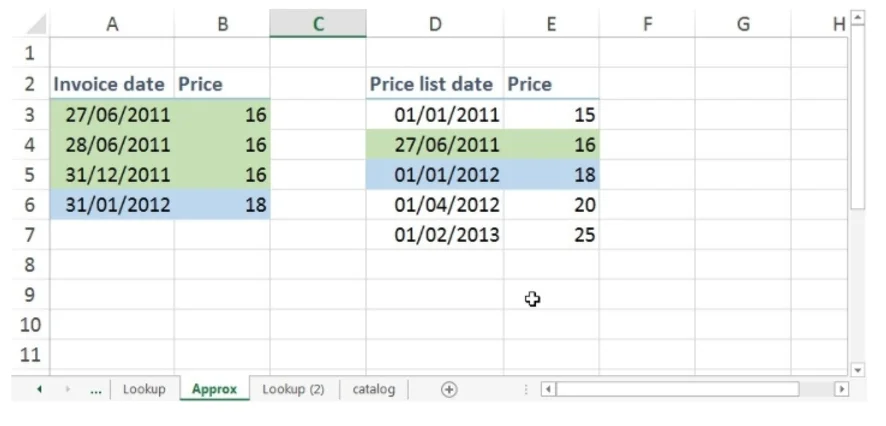
Say that we have a price list and we need to check the value of a particular product on a particular date:

Our price list just shows the date from which each new price came into use. Obviously, our invoice dates would not necessarily be just on those dates, so we would need to find the latest date (largest) that is smaller than or equal to our invoice date, which is what the approximate match will do as long as our price list table is sorted in ascending order of date.
HLOOKUP()
We can also use the example to show that HLOOKUP() is just the horizontal equivalent of VLOOKUP(), with the third argument referring to which row to use rather than which column:

INDEX MATCH
VLOOKUP() and HLOOKUP() can be very useful, but sometimes you want to look up data that isn’t organised left to right or work with values sorted in descending, rather than ascending, order. The combination of the MATCH() and INDEX() functions can help you do so.
MATCH() and INDEX() Although there are lots of similarities in the way that VLOOKUP() and HLOOKUP() work when compared with MATCH() and INDEX(), there are some important differences.
VLOOKUP() and HLOOKUP() return the value in a cell directly; MATCH() uses a similar approach to finding the matching cell as the lookup functions but doesn’t return the value, instead, it returns the position of the cell in the list of cells. As we will see, this is why MATCH() is often used with INDEX().
Also, the lookups can use a whole table of data and allow you to specify which column or row to use, MATCH() just works with a simple list: cells in a single column or in a single row.
MATCH() and INDEX() Together
Usually, in order to make use of MATCH() we need to use the value to retrieve the contents of the cell. This is why we need to combine MATCH() with INDEX(). INDEX() has two forms – we will look at the ‘array’ form here. In this context, array just means a block of cells rather than requiring the use of Control+Shift+Enter to create an actual array formula. At its simplest, INDEX() and MATCH() can be used to replace VLOOKUP() or HLOOKUP().
INDEX() takes three arguments: the block of cells that contains our table of values, a row number and an optional column number that define which cell within our block to return the value from.
Let’s look at an example:
To find the value for our 31/01/12 date we would use:
=INDEX($E$3:$F$7,B6,2)

This takes the value that our MATCH() function found and uses it as the row number, with the column number specifying that we should return the value from the second column of our table of data. We could have included the MATCH() function within the INDEX() function to do it all in one cell:
=INDEX($E$3:$F$7,MATCH(A6,$E$3:$E$7),2)
It’s that simple! Next time you need to look something up, try a VLOOKUP/HLOOKUP and an INDEX MATCH to see which works best for you.


